In this article, we will show how we can derive a generic circuit for probability distribution functions. Let a quantum system be described by the state

\[|\Psi\rangle = a|0\rangle + b|1\rangle\]

According the quantum theory, if we measure this system, we can find it in state $|0\rangle$ with probability $|a|^2$ and in state $|1\rangle$ with probability $|b|^2$, where $a$ and $b$ are complex numbers and $|a|^2 + |b|^2 = 1$.

Suppose $a$ and $b$ are real numbers, $f(x)$ a probability distribution with $x=\{0,1\}$ and $f(0) = a^2$ and $f(1) = b^2$, then we can write $|\Psi\rangle$ as

\[|\Psi\rangle = \sqrt{f(0)}|0\rangle + \sqrt{f(1)}|1\rangle\]

In general, if we have $n$ qubits and the domain of $f(x)$ is $0,1,2,\ldots 2^n-1$, then we can write $|\Psi\rangle$ as

\[|\Psi\rangle = \sum_{x=0}^{2^n-1} \sqrt{f(x)}|x\rangle\]

If the distribution is continuous, we will need to discretize it and map it to the intervals generated by $n$ qubits. We will show this later in the example on Lognormal distribution.

Probability Distributions on 2-Qubits

If we have two qubits, then the following table summarizes the possibilities:

\[\begin{array}{cccc} q_1\downarrow & q_0\rightarrow & 0 & 1 \\ 0 & & 00 & 01 \\ 1 & & 10 & 11 \end{array}\]

Let $P_0$ be the probability of the first qubit to have a value of 0 and $P_1$ be the probability of the first qubit to have a value of 1. Then according to the above table

\[\begin{array}{rl} P_0 &= P_{00} + P_{10} \\ P_1 &= P_{01} + P_{11} \end{array}\]

where $P_{ij}$ is the probability of getting the state $|ij\rangle$.

Define the following

\[\begin{array}{rl} f(0) &= P_{00}\\ f(1) &= P_{01}\\ f(2) &= P_{10}\\ f(3) &= P_{11} \end{array}\]

Then we can write the probability distribution for this system as:

\[\begin{array}{rl} |\Psi\rangle &= \sqrt{P_{00}}|00\rangle + \sqrt{P_{01}}|01\rangle + \sqrt{P_{10}}|10\rangle + \sqrt{P_{11}}|11\rangle \end{array}\]

Deriving the Circuit

We will now derive a circuit for this probability distribution. We are going to use the $RY(\theta)$ gate defined by

\[RY(\theta) = \left( \begin{array}{cc} \cos(\theta/2) & -\sin(\theta/2)\\ \sin(\theta/2) & \cos(\theta/2) \end{array} \right)\]

The action of $RY(\theta)$ on the state $|0\rangle$ is

\[RY(\theta) = \left( \begin{array}{cc} \cos(\frac{\theta}{2}) & -\sin(\frac{\theta}{2})\\ \sin(\frac{\theta}{2}) & \cos(\frac{\theta}{2}) \end{array} \right)\left( \begin{array}{c} 1\\ 0 \end{array} \right) = \cos(\frac{\theta}{2}) |0\rangle + \sin(\frac{\theta}{2})|1\rangle\]

Now that we have defined the $RY(\theta)$ gate, let’s define the following mappings:

\[\sqrt{P_0} = \cos(\theta_0)\]

From this we have

\[\begin{array}{rl} P_0 &= \cos^2(\theta_0)\\ &= 1-\sin^2(\theta_0)\\ 1-P_0 &= \sin^2(\theta_0) \\ P_1 &= \sin^2(\theta_0) \\ \end{array}\]

Therefore

\[\sqrt{P_1} = \sin(\theta_0)\]

Furthermore,

\[\begin{align} P_0 &= P_{00} + P_{10} \\ 1 &= \frac{P_{00}}{P_0} + \frac{P_{10}}{P_0} \end{align}\]

If we define

\[\sqrt{\frac{P_{00}}{P_0}} = \cos\frac{\theta_1}{2}\]

then

\[\begin{align} 1 &= \frac{P_{00}}{P_0} + \frac{P_{01}}{P_0} \\ &= \cos^2\frac{\theta_1}{2} + \frac{P_{01}}{P_0}\\ \frac{P_{01}}{P_0} &= 1- \cos^2\frac{\theta_1}{2} = \sin^2\frac{\theta_1}{2} \end{align}\]

Therefore,

\[\sqrt{\frac{P_{01}}{P_0}} = \sin\frac{\theta_1}{2}\]

In the same manner, we have

\[\begin{align} \sqrt{\frac{P_{10}}{P_1}} &= \cos\frac{\theta_2}{2}\\ \sqrt{\frac{P_{11}}{P_1}} &= \sin\frac{\theta_2}{2} \end{align}\]

Now we can write our probability distribution as:

\[|\Psi\rangle = \sqrt{P_0}\sqrt{\frac{P_{00}}{P_0}}|00\rangle + \sqrt{P_0}\sqrt{\frac{P_{01}}{P_0}}|01\rangle + \sqrt{P_1}\sqrt{\frac{P_{10}}{P_1}}|10\rangle + \sqrt{P_{11}}\sqrt{\frac{P_{11}}{P_{11}}}|11\rangle\]

Subsituting the values we derived earlier, we get

\[\begin{array}{rl} =&\left[\cos \frac{\theta_0}{2} \cos \frac{\theta_1}{2}|0\rangle|0\rangle + \cos\frac{\theta_0}{2}\sin\frac{\theta_1}{2}|0\rangle|1\rangle \right] + \underbrace{\left[\sin\frac{\theta_0}{2}\cos\frac{\theta_2}{2}|1\rangle|0\rangle + \sin\frac{\theta_0}{2}\sin\frac{\theta_2}{2}|1\rangle|1\rangle \right]}\\ \end{array}\]

The term in the underbrace can be factored to get

\[=\left[\cos \frac{\theta_0}{2} \cos \frac{\theta_1}{2}|0\rangle|0\rangle + \cos\frac{\theta_0}{2}\sin\frac{\theta_1}{2}|0\rangle|1\rangle \right] + \sin\frac{\theta_0}{2}|1\rangle\underbrace{\left[\cos\frac{\theta_2}{2}|0\rangle + \sin\frac{\theta_2}{2}|1\rangle \right]}\\\]

We can recognize that the term in the underbrace is the result of apply $RY(\theta_2)$ to $|0\rangle$

\[=\left[\cos \frac{\theta_0}{2} \cos \frac{\theta_1}{2}|0\rangle|0\rangle + \cos\frac{\theta_0}{2}\sin\frac{\theta_1}{2}|0\rangle|1\rangle \right] + \sin\frac{\theta_0}{2}|1\rangle\otimes RY(\theta_2)|0\rangle\\\]

We can factor out the $RY(\theta)2)$ as a controlled $RY(\theta_2)$ gate:

\[\begin{array}{rl} =&\mathrm{CRY}(\theta_2) \left[\cos \frac{\theta_0}{2} \cos \frac{\theta_1}{2}|0\rangle|0\rangle + \cos\frac{\theta_0}{2}\sin\frac{\theta_1}{2}|0\rangle|1\rangle + \sin\frac{\theta_0}{2}|1\rangle|0\rangle \right] \\ \end{array}\]

We can factor the terms in the underbrace to expose an $RY$ gate:

\[\begin{array}{rl} =&\mathrm{CRY}(\theta_2) \left[\underbrace{\cos \frac{\theta_0}{2} \cos \frac{\theta_1}{2}|0\rangle|0\rangle + \cos\frac{\theta_0}{2}\sin\frac{\theta_1}{2}|0\rangle|1\rangle} + \sin\frac{\theta_0}{2}|1\rangle|0\rangle \right] \\ =&\mathrm{CRY}(\theta_2) \left[\cos \frac{\theta_0}{2} |0\rangle\left(\underbrace{\cos \frac{\theta_1}{2}|0\rangle + \sin\frac{\theta_1}{2}|1\rangle}\right) + \sin\frac{\theta_0}{2}|1\rangle|0\rangle \right] \\ =&\mathrm{CRY}(\theta_2) \left[\cos \frac{\theta_0}{2} |0\rangle\otimes RY(\theta_1)|0\rangle + \sin\frac{\theta_0}{2}|1\rangle|0\rangle \right] \\ \end{array}\]

Notice that we can factor this $RY$ gate as a controlled $RY$ gate if we first flip the first qubits:

\[\begin{array}{rl} =&\mathrm{CRY}(\theta_2) \cdot X\otimes I \cdot \left[\cos \frac{\theta_0}{2} |1\rangle\otimes RY(\theta_1)|0\rangle + \sin\frac{\theta_0}{2}|0\rangle|0\rangle \right] \\ =&\mathrm{CRY}(\theta_2) \cdot X\otimes I \cdot \mathrm{CRY}(\theta_1) \left[\underbrace{\cos \frac{\theta_0}{2} |1\rangle|0\rangle + \sin\frac{\theta_0}{2}|0\rangle|0\rangle} \right] \\ \end{array}\]

We can factor out the righmost $|0\rangle$ qubit in the underbrace

\[\begin{array}{rl} =&\mathrm{CRY}(\theta_2) \cdot X\otimes I \cdot \mathrm{CRY}(\theta_1) \left[\left(\underbrace{\cos \frac{\theta_0}{2} |1\rangle + \sin\frac{\theta_0}{2}|0\rangle}\right) |0\rangle\right] \\ \end{array}\]

The terms in the underbrace looks like a $RY$ gate but we have to flip the qubits first by adding the gate $X\otimes I$ \(\begin{array}{rl} =&\mathrm{CRY}(\theta_2) \cdot X\otimes I \cdot \mathrm{CRY}(\theta_1)\cdot X\otimes I \left[\left(\underbrace{\cos \frac{\theta_0}{2} |0\rangle + \sin\frac{\theta_0}{2}|1\rangle}\right) |0\rangle\right] \\ \end{array}\)

Finally, we have derived the gate for a two qubit probability distribution:

\[\begin{array}{rl} =&\mathrm{CRY}(\theta_2) \cdot X\otimes I \cdot \mathrm{CRY}(\theta_1)\cdot X\otimes I \left[\left(\underbrace{RY(\theta_0)|0\rangle}\right) |0\rangle\right] \\ =&\mathrm{CRY}(\theta_2) \cdot X\otimes I \cdot \mathrm{CRY}(\theta_1)\cdot X\otimes I \cdot RY(\theta_0)|0\rangle |0\rangle\\ \end{array}\]

# Import the Qiskit SDK
from qiskit import QuantumCircuit, ClassicalRegister, QuantumRegister
from qiskit import execute, Aer
import numpy as np

# Create the input Quantum Register with 2 qubits.
qin = QuantumRegister(2)

# Create a Classical Register with 2 bits that will hold the result of the measurement
c = ClassicalRegister(2)

# Create the Quantum Circuit
qc = QuantumCircuit(qin,c)

# compute the angles
P00=<input>
P01=<input>
P10=<input>
P11=<input>
    
P0=P00+P10
P1=P01+P11
    
theta0 = 2*np.arccos(np.sqrt(P0))
theta1 = 2*np.arccos(np.sqrt(P00/P0))
theta2 = 2*np.arccos(np.sqrt(P01/P0))

print(theta0)
print(theta1)
print(theta2)

# Implement the circuit
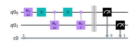
qc.ry(theta0, qin[0])
qc.x(qin[0])
qc.cry(theta1,qin[0],qin[1])
qc.x(qin[0])
qc.cry(theta2,qin[0],qin[1])

qc.barrier()  

# Measure and draw
qc.measure(qin,c)
qc.draw(output='mpl',interactive=True)

Here is how the circuit will look like:

Example: Uniform Distribution

A 2-qubit system will allow us to create 4-bins. Since this is uniform distribution, each bin will have the same probability of occuring, that is

\[P_{ij} = 1/4\]

for all $i,j \in \{0,1\}$

This means that

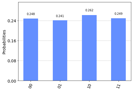
\[\begin{align} P_0 &= P_{00}+P_{10} = 0.5\\ P_1 &= P_{01}+P_{11} = 0.5\\ P_{00} &= 0.25\\ P_{01} &= 0.25 \end{align}\]

Plugging in these values in the above code and simulating we get:

Example: Sum of Quantum 2-dice

Suppose we have 2 dice with each die having 2 faces whose value can be 0 or 1. We throw the dice and examine the face that shows when they land. Whatever is the value, we take the sum. The question is what value of the sum is most probable?

We can tabulate the possible sums of 2-dices as follows where the values of the sum correspond to their binary representation.

\[\begin{array}{|r|r|l|}\hline & 0 & 1 \\\hline 0 & 00 & 01 \\\hline 1 & 01 & 10 \\\hline \end{array}\]

For example, if die 1 and die 2 come up as 1 and 1, then the sum is equal to 2 which is 10 in binary.

From the table above, we can compute the following probabilities:

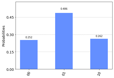
\[\begin{array}{rl} P_{00} &= 0.25\\ P_{01} &= 0.5 \\ P_{10} &= 0.25 \\ P_0 &= P_{00} + P_{01} = 0.25 + 0.25 = 0.5\\ P_1 &= P_{01} + P_{11} = 0.5 + 0 \end{array}\]

Note: There is no value = 11, so $P_{11} = 0$.

Example: LogNormal Distribution

The lognormal distribution is defined as

\[f(x) = \frac{1}{x\sigma\sqrt{2\pi}}\exp\left(-\frac{(\ln x - \mu)^2}{2\sigma^2}\right)\]

where $\mu$ is the mean and $\sigma^2$ is the variance.

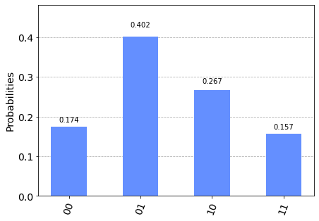
Using values $\mu=0$ and $\sigma=1$, create 4 bins with the following boundaries $0, 0.25, 0.5, 0.75, 1.0$ and get the probabilities from the lognormal cumulative distribution for each bin. The following are the probabilities:

\[\begin{align} P_{00}&=0.1656570 \\ P_{01}&=0.3225602 \\ P_{10}&=0.2853729 \\ P_{11}&=0.2264099 \end{align}\]

We have learned how to derive a generic 2-qubit circuit for a probability distribution. We validated the circuit using the uniform distribution and it is what we expected it to be. We have also shown the simulation for 2 other distributions. A challenge is to derive the circuit for a 3-qubit system, and for an n-qubit system. The number of gates is expected to be exponential on the number of qubits. That would be a further challenge for the interested person.

Image Credit: “From Above (Explored)” by Derek Giovanni Photography is licensed under CC BY-NC-ND 2.0. To view a copy of this license, visit https://creativecommons.org/licenses/by-nd-nc/2.0/jp/?ref=openverse.