A pre-sales person is covering a lot of cities and would like to travel to each city once and finally back to the originating city in such a way as to minimize the cost of fuel given that the more distance covered, the greater is the fuel consumed. This is the Traveling Salesman Problem (TSP). It is very popular since it is very hard to get an exact solution when the number of cities is large.
This is the second of a series of blogs that will talk about Variational Quantum Eigensolver (VQE). In this blog, we will show how to map the TSP to the Ising Model that will enable us to use the VQE to come up with an approximate solution to the TSP.
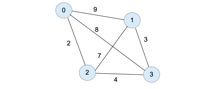
Let’s visualize this using the sample diagram below.
What you see is a graph representation of cities as nodes. Edges between nodes represent a route between them. Each edge has a weight which stands for the distance between the cities connected by this edge.
Suppose our pre-sales guy/girl wants to optimize the cost of fuel. He/She will need to list all possible routes and compute the total distance for each route. A route here is a closed route which begins with a certain city, visits the remaining cities once and returns to the starting city. Here is a listing of all possible routes (and total distance of that route) given the above graph:
\[\begin{array}{cccccc} 0 \rightarrow & 1 \rightarrow & 2 \rightarrow & 3 \rightarrow & 0 & \text{ dist = }28\\ 0 \rightarrow & 1 \rightarrow & 3 \rightarrow & 2 \rightarrow & 0 & \text{ dist = }18\\ 0 \rightarrow & 2 \rightarrow & 1 \rightarrow & 3 \rightarrow & 0 & \text{ dist = }20\\ 0 \rightarrow & 2 \rightarrow & 3 \rightarrow & 1 \rightarrow & 0 & \text{ dist = }18\\ 0 \rightarrow & 3 \rightarrow & 1 \rightarrow & 2 \rightarrow & 0 & \text{ dist = }20\\ 0 \rightarrow & 3 \rightarrow & 2 \rightarrow & 1 \rightarrow & 0 & \text{ dist = }28\\ 1 \rightarrow & 0 \rightarrow & 2 \rightarrow & 3 \rightarrow & 1 & \text{ dist = }18\\ 1 \rightarrow & 0 \rightarrow & 3 \rightarrow & 2 \rightarrow & 1 & \text{ dist = }28\\ 1 \rightarrow & 2 \rightarrow & 0 \rightarrow & 3 \rightarrow & 1 & \text{ dist = }20\\ 1 \rightarrow & 2 \rightarrow & 3 \rightarrow & 0 \rightarrow & 1 & \text{ dist = }28\\ 1 \rightarrow & 3 \rightarrow & 0 \rightarrow & 2 \rightarrow & 1 & \text{ dist = }20\\ 1 \rightarrow & 3 \rightarrow & 2 \rightarrow & 0 \rightarrow & 1 & \text{ dist = }18\\ \end{array}\] \[\begin{array}{cccccc} 2 \rightarrow & 0 \rightarrow & 1 \rightarrow & 3 \rightarrow & 2 & \text{ dist = }18\\ 2 \rightarrow & 0 \rightarrow & 3 \rightarrow & 1 \rightarrow & 2 & \text{ dist = }20\\ 2 \rightarrow & 1 \rightarrow & 0 \rightarrow & 3 \rightarrow & 2 & \text{ dist = }28\\ 2 \rightarrow & 1 \rightarrow & 3 \rightarrow & 0 \rightarrow & 2 & \text{ dist = }20\\ 2 \rightarrow & 3 \rightarrow & 0 \rightarrow & 1 \rightarrow & 2 & \text{ dist = }28\\ 2 \rightarrow & 3 \rightarrow & 1 \rightarrow & 0 \rightarrow & 2 & \text{ dist = }18\\ 3 \rightarrow & 0 \rightarrow & 1 \rightarrow & 2 \rightarrow & 3 & \text{ dist = }28\\ 3 \rightarrow & 0 \rightarrow & 2 \rightarrow & 1 \rightarrow & 3 & \text{ dist = }20\\ 3 \rightarrow & 1 \rightarrow & 0 \rightarrow & 2 \rightarrow & 3 & \text{ dist = }18\\ 3 \rightarrow & 1 \rightarrow & 2 \rightarrow & 0 \rightarrow & 3 & \text{ dist = }20\\ 3 \rightarrow & 2 \rightarrow & 0 \rightarrow & 1 \rightarrow & 3 & \text{ dist = }18\\ 3 \rightarrow & 2 \rightarrow & 1 \rightarrow & 0 \rightarrow & 3 & \text{ dist = }28\\ \end{array}\]From the result above, we can see that the shortest path has a total distance of 18 units.
Cost to Minimize
The closed routes in the Traveling Salesman problem are called Hamiltonian routes. It is specified by $N^2$ binary variables $x_{i,p}$, where $i$ is the ith city and $p$ is the order of the city for a given instance of a route.
For example, a route
\[2 \rightarrow 3 \rightarrow 1 \rightarrow 0\]is represented by
\[\begin{array}{c|cccc} & 0 & 1 & 2 & 3\\\hline 0 & 0 & 0 & 0 & 1\\ 1 & 0 & 0 & 1 & 0\\ 2 & 1 & 0 & 0 & 0\\ 3 & 0 & 1 & 0 & 0\\ \end{array}\]The rows represent the city and the columns represent the position of the node in the current route. To determine the position of a city in a given route, find the row of the city and find the column that contains the value 1. Each cell of the matrix is a variable $x_{i,p}$ and has a value of either 1 or 0.
Note: Although we did not state explicitly, the route ends in the starting city. So in this example, after visiting city 0, the traveller will go back to city 2.
Notice that in the above matrix, we have the following constraints:
\[\displaystyle \sum_p x_{i,p} = 1 \text{ for all }i\]and
\[\displaystyle \sum_i x_{i,p} = 1 \text{ for all }p\]We can “unpack” this matrix into a vector $x=[x_1,x_2,\ldots,x_{N^2}]$ such that $x_j = x_{N\cdot i + p}$, where $N$ is the number of cities. So in our example, we have $N=4$ and the variable $x_{2,1}$, maps to $x_9$. An instance of this vector is a route. Using this representation, the route
\[2 \rightarrow 3 \rightarrow 1 \rightarrow 0\]which is represented by
\[\begin{array}{c|cccc} & 0 & 1 & 2 & 3\\\hline 0 & 0 & 0 & 0 & 1\\ 1 & 0 & 0 & 1 & 0\\ 2 & 1 & 0 & 0 & 0\\ 3 & 0 & 1 & 0 & 0\\ \end{array}\]becomes the vector
\[x=[0,0,0,1,0,0,1,0,1,0,0,0,0,1,0,0]\]Later, we will see that this is an eigenstate when we map the TSP to the Ising Model.
If we let $w_{i,j}$ be the distance between city i and city j, then the total distance for each route is given by
\[\displaystyle \sum_{i,j} w_{i,j}\sum_p x_{i,p}x_{j,p+1}\]If we add the constraints for the rows and columns, we get
\[\displaystyle \sum_{i,j} w_{i,j}\sum_p x_{i,p}x_{j,p+1} + A \sum_p \left(\underbrace{ 1-\sum_i x_{i,p}}\right)^2 + A \sum_i\left(\underbrace{ 1-\sum_p x_{i,p}}\right)^2\]where the terms in underbraces are squared so that the lowest possible minimum value is zero. The factor $A$ can be chosen so that the constraints will be respected.
Mapping to the Ising Model
Our objective in this blog is to map this problem to the Ising Model so that it’s amenable to be solved using Quantum Computing.
First, we map the routes $x=[x_1, x_2, x_3, \ldots, x_{N^2}]$ to the $N^2$ qubits:
\[x=[x_1, x_2, x_3, \ldots, x_{N^2}] \rightarrow |\psi\rangle=|x_1\rangle\otimes|x_2\rangle\cdots\otimes|x_{N^2}\rangle\]Next, we map the cost function above to the Ising Model using the following change of variables:
\[x_{i,p} \rightarrow \displaystyle \frac{1-Z_{i,p}}{2}\]where $Z$ is the Pauli Z operator.
See Appendix to see a sample of how terms expand.
By mapping this to the Ising Model, this becomes an eigenvalue problem
\[H|\psi\rangle = k|\psi\rangle\]where $H$ is the Ising Hamiltonian and $\vert\psi\rangle$ is the eigenstate corresponding to the eigenvalue $k$. The eigenstate corresponds to the state $\vert\psi\rangle=\vert x_1\rangle\otimes\vert x_2\rangle\cdots\otimes\vert x_{N^2}\rangle$. By finding the eigenstate that corresponds to the minimum eigenvalue, we will be able to solve our problem.
We can easily do this mapping using the IBM QISKit tsp module.
An Example Using QISKit
For a TSP problem with N cities, the number of qubits is equal to $N^2$. The number of basis states corresponding to this is $2^N$. For a 4-city problem, the number of qubits is $4^2 = 16$ and the number of states is $2^{16}=65536$. Because of this, we just give an example of 3 cities.
Suppose we have the following distance matrix for 3 cities:
\[W=\left( \begin{array}{ccc} 0 & 78 & 45 \\ 78 & 0 & 100 \\ 45 & 100 & 0 \\ \end{array} \right)\]Using IBM QisKit, we can map this to the Ising model using the get_tsp_qubitops method of the tsp class:
import numpy as np
import qiskit.aqua.translators.ising.tsp as tsp
from qiskit.aqua.algorithms import VQE, ExactEigensolver
from qiskit.aqua.translators.ising.tsp import TspData

w=[[  0.,  78., 45.],[ 78., 0., 100.],[ 45., 100.,  0.]]

np.array(w)

tspdata=TspData("tmp", 3, [], w=np.array(w))
qubitOp, offset = tsp.get_tsp_qubitops(tspdata)
The variable qubitOp is an Operator object and represents the Hamiltonian of the system (not to be confused by the Hamiltonian circuit of the TSP).
Here is the code to solve this problem using the ExactEigensolver (lifted from the Jupyter notebook of the TSP tutorial in QISKit):
ee = ExactEigensolver(qubitOp, k=1)
result = ee.run()

"""
algorithm_cfg = {
    'name': 'ExactEigensolver',
}

params = {
    'problem': {'name': 'ising'},
    'algorithm': algorithm_cfg
}
result = run_algorithm(params,algo_input)
"""
print('energy:', result['energy'])
x = tsp.sample_most_likely(result['eigvecs'][0])
print('feasible:', tsp.tsp_feasible(x))
z = tsp.get_tsp_solution(x)
print('solution:', z)
print('solution objective:', tsp.tsp_value(z, tspdata.w))
Executing the code above using gives a solution to the TSP:
energy: -600111.5
feasible: True
solution: [0, 1, 2]
solution objective: 223.0
Conclusion
We have not yet discussed the Variational Quantum Eigensolver (VQE). That will be the last topic in this series. What we have done is understand how the TSP is mapped into the Ising Problem. We then used the ExactEigensolver to find the minimum eigenvalue that will correspond to a solution to the problem. In the next blog, we will show how the VQE can be used to get an approximation of a solution to the TSP problem after mapping it to the Ising Model.
Appendix
Mapping the TSP to the Ising model involves transforming the cost function
\[\displaystyle \sum_{i,j} w_{i,j}\sum_p x_{i,p}x_{j,p+1} + A \sum_p \left(\underbrace{ 1-\sum_i x_{i,p}}\right)^2 + A \sum_i\left(\underbrace{ 1-\sum_p x_{i,p}}\right)^2\]using
\[x_{i,p} \rightarrow \displaystyle \frac{1-Z_{i,p}}{2}\]where $Z$ is the Pauli Z operator.
As an example, for $p={0,1,2}$, the second term above will look like:
\[\begin{array}{rl} \displaystyle \sum_p \left( 1-\sum_i x_{i,p}\right)^2 &= \displaystyle \sum_p\left(1-\sum_i \frac{1-Z_{i,p}}{2}\right)^2\\ &= \displaystyle-\frac{1}{2} \sum_p \left(\underbrace{1 - Z_{0,p}-Z_{1,p}-Z_{2,p} }\right)^2\\ \end{array}\]We can expand the square as
\[-2Z_{0,p} -2Z_{1,p} -2Z_{2,p} + Z_{0,p}Z_{1,p} + Z_{0,p}Z_{2,p} + Z_{1,p}Z_{0,p} + Z_{1,p}Z_{2,p} + Z_{2,p}Z_{0,p}+Z_{2,p}Z_{1,p}\]For a given p, say p=0, we have:
\[\begin{array}{rl} & -2Z_{0,p} -2Z_{1,p} -2Z_{2,p} + Z_{0,p}Z_{1,p} + Z_{0,p}Z_{2,p} + Z_{1,p}Z_{0,p} + Z_{1,p}Z_{2,p} + Z_{2,p}Z_{0,p}+Z_{2,p}Z_{1,p}\\ &= -2Z_{0,0} -2Z_{1,0} -2Z_{2,0} + Z_{0,0}Z_{1,0} + Z_{0,0}Z_{2,0} + Z_{1,0}Z_{0,0} + Z_{1,0}Z_{2,0} + Z_{2,0}Z_{0,0}+Z_{2,0}Z_{1,0} \\ &= -2Z_0 -2Z_3 -2Z_6 + Z_0Z_3 + Z_0Z_6 + Z_3Z_0 + Z_3Z_6 + Z_6Z_0 + Z_6Z_3\\ &= -2Z_0 -2Z_3 -2Z_6 + 2Z_0Z_3 + 2Z_0Z_6 + 2Z_3Z_6\\ &= -(Z_0 + Z_3 - 2Z_0Z_3 ) - (Z_0 + Z_6 - 2Z_0Z_6) - (Z_3 + Z_6 - Z_3Z_6) \end{array}\]Here is the code to generate the circuit for the above expansion (taken from the tsp source code):
    for p in range(num_nodes):
        for i in range(num_nodes):

            for j in range(i):
                print("p= ", p, " i=", i, "j=",j)
                shift += penalty / 2

                zp = np.zeros(num_qubits, dtype=np.bool)
                zp[i * num_nodes + p] = True
                print(i*num_nodes + p)
                pauli_list.append([-penalty / 2, Pauli(zp, zero)])

                zp = np.zeros(num_qubits, dtype=np.bool)
                zp[j * num_nodes + p] = True
                print(j*num_nodes + p)
                pauli_list.append([-penalty / 2, Pauli(zp, zero)])

                zp = np.zeros(num_qubits, dtype=np.bool)
                zp[i * num_nodes + p] = True
                zp[j * num_nodes + p] = True

                pauli_list.append([penalty / 2, Pauli(zp, zero)])
If you print the pauli_list, you will get the following:
IIIIIZIII -> Z3
IIIIIIIIZ -> Z0
IIIIIZIIZ -> Z3Z0
IIZIIIIII -> Z6
IIIIIIIIZ -> Z0
IIZIIIIIZ -> Z6Z0
IIZIIIIII -> Z6
IIIIIZIII -> Z3
IIZIIZIII -> Z3Z6
This matches our expansion above.
Image Credit: “Travelling Salesman” by MeoplesMagazine is marked with CC BY-NC-SA 2.0. To view the terms, visit https://creativecommons.org/licenses/by-nc-sa/2.0/?ref=openverse
 Bobby Corpus


 I Sing Quantum Computing