 Bobby Corpus
In the last post (Quantum Searching), we saw how quantum search works even without a quantum computer. In this post, we will see how to program the search using the IBM QISKit.
The goal in quantum search is to find the value $a$ such that given a function $f(x)$, the value of $f$ is equal to 1 when $x = a$. There can be more than one value of $a$ that satisfies this relationship.
| As we have seen here, searching for the state $\vert a\rangle$ is a matter of rotating the state $\vert \phi\rangle$, where $\vert \phi\rangle=1/\sqrt{2}^2 \sum_{x=0}^{2^n -1 } | x\rangle$. Therefore, the search process is computing for the vector |
so that
\[\langle a|\Psi\rangle \approx 0\]and then measuring the state $\vert \Psi\rangle$ to get the basis state that corresponds to the unknown $\vert a\rangle$.
To program this, we need to construct the circuits of both $\mathrm{V}$ and $\mathrm{W}$.
But first and foremost, let’s construct the $\vert\phi\rangle$ circuit.
The $\vert\phi\rangle$ Circuit
First, start with the n-qubit input state and 1 qubit output state $\vert 0…0\rangle\otimes\vert 1\rangle$ and create a superposition of states using the hadamard operator:
\[\mathrm{H}^{\otimes n}|0...0\rangle \otimes\mathrm{H}|1\rangle = |\phi\rangle\otimes\mathrm{H}|1\rangle = \displaystyle \frac{1}{\sqrt{2}^n} \sum_{x=0}^{2^{n}-1} |x\rangle\otimes \mathrm{H}|1\rangle\]This is equivalent to the circuit:

The $\mathrm{V}$ Circuit
Constructing the $\mathrm{V}$ circuit is equivalent to constructing the $\mathrm{U}_f$ circuit.
Apply the unitary operator $\mathrm{U}_f$ to the state $\vert \phi\rangle$:
\[\mathrm{U}_f\Big[|\phi\rangle\otimes \mathrm{H}|1\rangle\Big] = \displaystyle \frac{1}{\sqrt{2}^n} \sum_{x=0}^{2^{n}-1} (-1)^{f(x)} |x\rangle\otimes \mathrm{H}|1\rangle\]The $\mathrm{U}_f$ circuit, shown below in a red box, returns 1 for $\vert x\rangle = \vert 6\rangle \equiv \vert 110_2\rangle$ and 0 otherwise

Constructing the $\mathrm{U}_f$ Circuit
So how do we check if the input qubits are in the state $\vert 110\rangle$ ?
- Initialize all auxiliary qubits to the $\vert 0\rangle$ state.
- Check if the first qubit is $\vert 0\rangle$. To check this, negate it using the $\mathrm{NOT}$ gate $\mathrm{X}$. Then using the CNOT gate, this will put qubit $\mathrm{aux1}_1$ in the state $\vert 1\rangle$ if the first qubit is $\vert 0\rangle$.
- Next, check that the 2nd and 3rd input qubits are in the state $\vert 1\rangle$ using the Controlled-CNOT gate. If both are in state $\vert 1\rangle$, then the qubit $\mathrm{aux1}_0$ will become $\vert 1\rangle$.
- Since both $\mathrm{aux1}_0$ and $\mathrm{aux1}_1$ are in the state $\vert 1\rangle$, this will flip the state of the output qubit $\mathrm{out1}_0$.
- Reset the values of the $\mathrm{aux1}$ qubits back to $\vert 0\rangle$ using the control gates on the right.
- Finally reset the value of the first qubit back to its original value using the $\mathrm{NOT}$ gate X at the far right.
Constructing the $W$ Circuit
The operator W is defined as
\[W=2|\phi\rangle\langle\phi| - \mathrm{I} = \mathrm{H}^{\otimes n}\Big[ 2|0\rangle\langle 0| - I\Big] \mathrm{H}^{\otimes n}\]It’s just a matter of constructing the circuit that implements $2\vert 0\rangle\langle 0\vert - \mathrm{I}$.
Let $\vert x\rangle$ be a basis vector. Then
\[\Big[ 2|0\rangle\langle 0| - \mathrm{I} \Big]|x\rangle = \begin{cases} -|x\rangle & x\ne 0\\ |0\rangle & x = 0 \end{cases}\]It is simpler to implement $\Big[\mathrm{I} - 2\vert 0\rangle\langle 0\vert \Big]$ since it acts as the identity for any basis vector not equal to $\vert 0\rangle$ and multiplies $\vert 0\rangle $ by -1. This means we will be implementing $-\mathrm{W}$, which is ok since the -1 factor will not have any impact when we take the probabilities.
To implement $\Big[\mathrm{I} - 2\vert 0\rangle\langle 0\vert \Big]$ as a circuit, we need one auxiliary qubit that will record if the first and second qubit are both in state $\vert 1\rangle$ using a Controlled-CNOT gate. Then a controlled-Z gate will negate the third qubit if the auxiliary qubit is in state $\vert 1\rangle$ and the third qubit is $\vert 1\rangle$.
In sequence of operations, first we have to negate the qubits to turn state $\vert 0\rangle$ to $\vert 1\rangle$. Then we do the sequence below:
\[\mathrm{CCNOT} \cdot \underbrace{|1\rangle}_{qin_0}\otimes\underbrace{|1\rangle}_{qin_1}\otimes\underbrace{|0\rangle}_{aux2_0} = |1\rangle\otimes|1\rangle\otimes\underbrace{|1\rangle}_{aux2_0}\] \[\mathrm{CtrlZ}\Big[\underbrace{|1\rangle}_{aux2_0}\underbrace{|1\rangle}_{qin_2}\Big]=-\underbrace{|1\rangle}_{aux2_0}\underbrace{|1\rangle}_{qin_2}\]Afterwards, we negate again the qubits to return them to previous state. The end result will be taking the state $\vert 0…0\rangle $ to $-\vert 0…0\rangle $. The diagram below is the implementation of this circuit. The Hadamards to the left and right make this the implementation of the $-\mathrm{W}$ circuit.

The full circuit
Now that we have $\mathrm{U}_f$ and $\mathrm{W}$, the full circuit is:

QISKit program
Finally, here is the code to implement the quantum search:
# Import the Qiskit SDK
from qiskit import QuantumCircuit, ClassicalRegister, QuantumRegister
from qiskit import execute, Aer
from qiskit.tools.visualization import circuit_drawer, plot_histogram

# function to apply hadamards to the input and output qubits
def h(qcirc, qin, qo):
    qcirc.h(qo[0])
    for i in range(0,3):
       qcirc.h(qin[i])

# function to return 1 when the state is 6 == 110 (base2)
def uf(qcirc, qin, aux1, qo):
    qcirc.ccx(qin[1],qin[2],aux1[0])
    qcirc.x(qin[0])
    qcirc.cx(qin[0],aux1[1])
    qcirc.ccx(aux1[0],aux1[1],qo[0])
    qcirc.cx(qin[0],aux1[1])
    qcirc.x(qin[0])
    qcirc.ccx(qin[1],qin[2],aux1[0])

# function that implements W
def w(qcirc,qin,qaux):
    for i in range(0,3):
        qcirc.h(qin[i])
        qc.x(qinput[i])

    qcirc.ccx(qinput[0],qinput[1],qaux[0])
    qcirc.cz(qaux[0],qinput[2])
    qcirc.ccx(qinput[0],qinput[1],qaux[0])

    qcirc.barrier()

    for i in range(0,3):
        qcirc.x(qinput[i])

    qcirc.barrier()

    for i in range(0,3):
        qcirc.h(qinput[i])

    qcirc.barrier()

# Define the Registers and circuit.
qx1 = QuantumRegister(2,name="aux1")
qout = QuantumRegister(1,name="qout")
qx = QuantumRegister(1,name="aux2")
qinput = QuantumRegister(3,name="qin")
coutput = ClassicalRegister(3,name="cout")
qc = QuantumCircuit(qinput,qout,coutput,qx1,qx)

# start computing. First negate the output register
qc.x(qout[0])
qc.barrier()

# Apply hadamards to the input and output
h(qc,qinput,qout)
qc.barrier()

# Apply the U_f operator
uf(qc,qinput,qx1,qout)
qc.barrier()

# Apply the W operator
w(qc,qinput,qx)
qc.barrier()

# Visualize the circuit.
from qiskit.tools.visualization import matplotlib_circuit_drawer as drawer, qx_color_scheme
my_style = {'plotbarrier': True}
my_scheme=qx_color_scheme()
my_scheme['plotbarrier'] = False
drawer(qc, style=my_scheme)

# Take a measurement
qc.measure(qinput,coutput)

# Compile and run the Quantum circuit on a simulator backend
backend_sim = Aer.get_backend('qasm_simulator')
shots = 1000

job_sim = execute(qc, backend=backend_sim, shots=shots)
result_sim = job_sim.result()
answer = result_sim.get_counts()
plot_histogram(answer)
And here is the result of the computation.

As you can see, the quantum computation was able to find our number with 77% probability. It seems that the accuracy is not that great at 77%. Actually, we can make it more accurate by applying the operator $\mathrm{WV}$ again:

In fact, we can apply $\mathrm{WV}$ up to $O(\sqrt{N})$ times, where $N=2^n$. See this post for more information.
Image Credit: “Search Technology Redux” by brewbooks is marked with CC BY-SA 2.0. To view the terms, visit https://creativecommons.org/licenses/by-sa/2.0/?ref=openverse
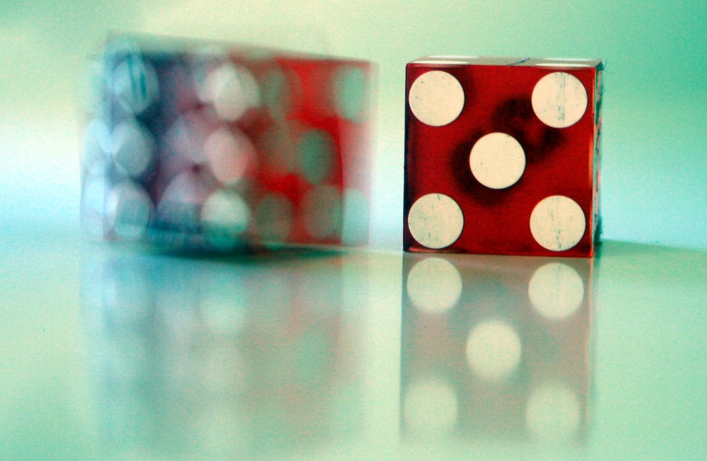 Quantum Computing: Programming the Quantum Dice