I have always been fascinated by computing. Thanks to my friends Ernesto Adorio (♱) and Augusto Hermosilla, both of whom are mathematicians, who introduced me to optimization. Ernie and I built the first MathNOW (Network of Workstations) in the University of the Philippines powered by Linux and MPI (Message Passing Interface). We then used this cluster to come up with a paper on Parallel Genetic Algorithms. This blog post is a first part of a series about how Quantum Computing is used to tackle NP-Complete problems.

Doing Quantum Computing is like creating musical scores as you can see from the image above. That’ s probably what inspired me to give this blog the title “I Sing Quantum Computing”.  Apart from that, this blog post is about the Ising Model of Quantum Physics.

The Ising model is a model to describe magnetic materials as a lattice of particles with spin-up or spin-down orientation. When a magnetic material such as iron is hot, the orientation of the spins is random. But when it cools, spins tend to form regions (called magnetic domains) such that the spins in each region is aligned. Each particle interacts with its nearest neighbor with a weight of $w_{ij} = w_{ji} $. The Hamiltonian (total energy) of the system of particles is given by

\[\displaystyle H= -\sum_{ij} w_{ij}\sigma_i\sigma_j\]

where $\sigma_i$ is either 1 or -1 representing the spin of the particle. From the hamiltonian, we can compute the minimum eigenvalue and the corresponding eigenstate. The eigenstate will correspond to the orientations of the spins of each particle.

Mapping NP-Complete Problems to the Ising Model

Consider a graph of N nodes and edges between nodes. Each edge has a weight $w_{ij}$ corresponding to the interaction between the nodes connected by the edge. Partition this graph into 2 subsets by assigning a value of 0 or 1 to each node. Get the total interaction of this partitioning by summing the interaction term for every edge that connects a node from subset 1 to subset 2, that is

\[\displaystyle C=\sum_{i,j} w_{i,j} x_i(1-x_j)\]

The total interaction $C$ is called the cost function. Now we want to find a subset such that the cost function is maximum. This is called the max-cut problem. It’s like cutting the graph into 2 subsets and maximizing the sum of the interaction terms of each edge that crosses the cut.

An Example: Maximum Cut

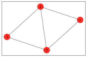
Suppose we have 4 nodes connected to each other in the following way and $w_{ij} = 1$:

Assign 0 or 1 to each node and compute the cost function C. An example assignment looks like:

\[(1,0,0,0)\]

Since node0 is connected to node1, node2 and node3, then we have

\[C=w_{01} + w_{02} + w_{03} = 1+1+1 = 3\]

Below are 16 possible ways to assign 0’s and 1’s and the corresponding value of the cost function computed using the above method:

\[\begin{array}{rl} (0, 0, 0, 0) &\text{cost} = 0.0\\ (1, 0, 0, 0) &\text{cost} = 3.0\\ (0, 1, 0, 0) &\text{cost} = 2.0\\ (1, 1, 0, 0) &\text{cost} = 3.0\\ (0, 0, 1, 0) &\text{cost} = 3.0\\ (1, 0, 1, 0) &\text{cost} = 4.0\\ (0, 1, 1, 0) &\text{cost} = 3.0\\ (1, 1, 1, 0) &\text{cost} = 2.0\\ (0, 0, 0, 1) &\text{cost} = 2.0\\ (1, 0, 0, 1) &\text{cost} = 3.0\\ (0, 1, 0, 1) &\text{cost} = 4.0\\ (1, 1, 0, 1) &\text{cost} = 3.0\\ (0, 0, 1, 1) &\text{cost} = 3.0\\ (1, 0, 1, 1) &\text{cost} = 2.0\\ (0, 1, 1, 1) &\text{cost} = 3.0\\ (1, 1, 1, 1) &\text{cost} = 0.0 \end{array}\]

From the above, the we can see that the cost function attains a maximum at (1,0,1,0) and (0,1,0,1) with a value of C=4.

The Mapping

We can map this to the Ising model in the following way. Let $Z$ be the Pauli Z operator defined by

\[\begin{array}{rl} Z|0\rangle &= |0\rangle\\ Z|1\rangle &= -|1\rangle \end{array}\]

Then by a change of variables

\[\displaystyle x_i \rightarrow \frac{1-Z_i}{2}\]

and remembering that $w_{ij} = w_{ji}$, we can transform C into:

\[\begin{array}{rl} \displaystyle C &=\displaystyle \sum_{i,j} w_{ij}\frac{1-Z_i}{2}\frac{1+Z_j}{2} \\ \displaystyle &= \displaystyle \sum_{i,j}\frac{w_{ij}}{4} + \sum_{i,j} \frac{w_{ij}}{4}Z_j -\sum_{i,j}\frac{w_{ij}}{4}Z_i -\sum_{i,j}w_{ij}Z_iZ_j\\ &= \displaystyle\sum_{i < j}\frac{w_{ij}}{2} - \sum_{i,j}w_{ij}Z_iZ_j\\ &= \displaystyle \text{Constant} - \sum_{i < j}\frac{w_{ij}}{2}Z_iZ_j \end{array}\]

Therefore, to maximize C, we need to minimize the Ising Hamiltonian:

\[\displaystyle H = \sum_{i<j}\frac{w_{ij}}{2}Z_iZ_j\]

Representing the Nodes as Qubits

Using qubits, we can represent an assignment of 0’s and 1’s as a tensor product of single qubits $\vert q_i\rangle$:

\[|q_3\rangle\otimes|q_2\rangle\otimes|q_1\rangle\otimes|q_0\rangle = |q_3\rangle|q_2\rangle|q_1\rangle|q_0\rangle = |q_3q_2q_1q_0\rangle\]

In this representation, the basis states are:

\[\begin{array}{l} |0000\rangle\\ |1000\rangle\\ |0100\rangle\\ |1100\rangle\\ |0010\rangle\\ |1010\rangle\\ |0110\rangle\\ |1110\rangle\\ |0001\rangle\\ |1001\rangle\\ |0101\rangle\\ |1101\rangle\\ |0011\rangle\\ |1011\rangle\\ |0111\rangle\\ |1111\rangle\\ \end{array}\]

In this basis, we can compute the matrix representation of $Z_0 $. Remember that $Z_i $ means that the Pauli Z operator operates on the ith qubit. For example,

\[Z_0 |0000\rangle = |0\rangle\otimes|0\rangle\otimes|0\rangle\otimes Z_0|0\rangle = |0000\rangle\]

In the same way,

\[Z_3 |1000\rangle = Z_3|1\rangle\otimes|0\rangle\otimes|0\rangle\otimes Z_0|0\rangle = -|1000\rangle\]

Given the above, we can now compute the matrix representation of $Z_0$ and is given by

\[Z_0=\left(\begin{array}{cccccccccccccccc} 1 & 0 & 0 & 0 & 0 & 0 & 0 & 0 & 0 & 0 & 0 & 0 & 0 & 0 & 0 & 0\\ 0 & -1 & 0 & 0 & 0 & 0 & 0 & 0 & 0 & 0 & 0 & 0 & 0 & 0 & 0 & 0\\ 0 & 0 & 1 & 0 & 0 & 0 & 0 & 0 & 0 & 0 & 0 & 0 & 0 & 0 & 0 & 0\\ 0 & 0 & 0 & -1 & 0 & 0 & 0 & 0 & 0 & 0 & 0 & 0 & 0 & 0 & 0 & 0\\ 0 & 0 & 0 & 0 & 1 & 0 & 0 & 0 & 0 & 0 & 0 & 0 & 0 & 0 & 0 & 0\\ 0 & 0 & 0 & 0 & 0 & -1 & 0 & 0 & 0 & 0 & 0 & 0 & 0 & 0 & 0 & 0\\ 0 & 0 & 0 & 0 & 0 & 0 & 1 & 0 & 0 & 0 & 0 & 0 & 0 & 0 & 0 & 0\\ 0 & 0 & 0 & 0 & 0 & 0 & 0 & -1 & 0 & 0 & 0 & 0 & 0 & 0 & 0 & 0\\ 0 & 0 & 0 & 0 & 0 & 0 & 0 & 0 & 1 & 0 & 0 & 0 & 0 & 0 & 0 & 0\\ 0 & 0 & 0 & 0 & 0 & 0 & 0 & 0 & 0 & -1 & 0 & 0 & 0 & 0 & 0 & 0\\ 0 & 0 & 0 & 0 & 0 & 0 & 0 & 0 & 0 & 0 & 1 & 0 & 0 & 0 & 0 & 0\\ 0 & 0 & 0 & 0 & 0 & 0 & 0 & 0 & 0 & 0 & 0 & -1 & 0 & 0 & 0 & 0\\ 0 & 0 & 0 & 0 & 0 & 0 & 0 & 0 & 0 & 0 & 0 & 0 & 1 & 0 & 0 & 0\\ 0 & 0 & 0 & 0 & 0 & 0 & 0 & 0 & 0 & 0 & 0 & 0 & 0 & -1 & 0 & 0\\ 0 & 0 & 0 & 0 & 0 & 0 & 0 & 0 & 0 & 0 & 0 & 0 & 0 & 0 & 1 & 0\\ 0 & 0 & 0 & 0 & 0 & 0 & 0 & 0 & 0 & 0 & 0 & 0 & 0 & 0 & 0 & -1\\ \end{array} \right)\]

Doing the same thing for $Z_1,Z_2,Z_3$, we can then compute the matrix for our Hamiltonian:

\[\displaystyle H = \sum_{i < j}\frac{w_{i < j}}{2}Z_iZ_j = \frac{z_{01} + z_{02} + z_{03} + z_{12} + z_{23}}{2}\]

to get

\[H=\left( \begin{array}{cccccccccccccccc} 2.5 & 0.0 & 0.0 & 0.0 & 0.0 & 0.0 & 0.0 & 0.0 & 0.0 & 0.0 & 0.0 & 0.0 & 0.0 & 0.0 & 0.0 & 0.0\\ 0.0 & -0.5 & 0.0 & 0.0 & 0.0 & 0.0 & 0.0 & 0.0 & 0.0 & 0.0 & 0.0 & 0.0 & 0.0 & 0.0 & 0.0 & 0.0\\ 0.0 & 0.0 & 0.5 & 0.0 & 0.0 & 0.0 & 0.0 & 0.0 & 0.0 & 0.0 & 0.0 & 0.0 & 0.0 & 0.0 & 0.0 & 0.0\\ 0.0 & 0.0 & 0.0 & -0.5 & 0.0 & 0.0 & 0.0 & 0.0 & 0.0 & 0.0 & 0.0 & 0.0 & 0.0 & 0.0 & 0.0 & 0.0\\ 0.0 & 0.0 & 0.0 & 0.0 & -0.5 & 0.0 & 0.0 & 0.0 & 0.0 & 0.0 & 0.0 & 0.0 & 0.0 & 0.0 & 0.0 & 0.0\\ 0.0 & 0.0 & 0.0 & 0.0 & 0.0 & -1.5 & 0.0 & 0.0 & 0.0 & 0.0 & 0.0 & 0.0 & 0.0 & 0.0 & 0.0 & 0.0\\ 0.0 & 0.0 & 0.0 & 0.0 & 0.0 & 0.0 & -0.5 & 0.0 & 0.0 & 0.0 & 0.0 & 0.0 & 0.0 & 0.0 & 0.0 & 0.0\\ 0.0 & 0.0 & 0.0 & 0.0 & 0.0 & 0.0 & 0.0 & 0.5 & 0.0 & 0.0 & 0.0 & 0.0 & 0.0 & 0.0 & 0.0 & 0.0\\ 0.0 & 0.0 & 0.0 & 0.0 & 0.0 & 0.0 & 0.0 & 0.0 & 0.5 & 0.0 & 0.0 & 0.0 & 0.0 & 0.0 & 0.0 & 0.0\\ 0.0 & 0.0 & 0.0 & 0.0 & 0.0 & 0.0 & 0.0 & 0.0 & 0.0 & -0.5 & 0.0 & 0.0 & 0.0 & 0.0 & 0.0 & 0.0\\ 0.0 & 0.0 & 0.0 & 0.0 & 0.0 & 0.0 & 0.0 & 0.0 & 0.0 & 0.0 & -1.5 & 0.0 & 0.0 & 0.0 & 0.0 & 0.0\\ 0.0 & 0.0 & 0.0 & 0.0 & 0.0 & 0.0 & 0.0 & 0.0 & 0.0 & 0.0 & 0.0 & -0.5 & 0.0 & 0.0 & 0.0 & 0.0\\ 0.0 & 0.0 & 0.0 & 0.0 & 0.0 & 0.0 & 0.0 & 0.0 & 0.0 & 0.0 & 0.0 & 0.0 & -0.5 & 0.0 & 0.0 & 0.0\\ 0.0 & 0.0 & 0.0 & 0.0 & 0.0 & 0.0 & 0.0 & 0.0 & 0.0 & 0.0 & 0.0 & 0.0 & 0.0 & 0.5 & 0.0 & 0.0\\ 0.0 & 0.0 & 0.0 & 0.0 & 0.0 & 0.0 & 0.0 & 0.0 & 0.0 & 0.0 & 0.0 & 0.0 & 0.0 & 0.0 & -0.5 & 0.0\\ 0.0 & 0.0 & 0.0 & 0.0 & 0.0 & 0.0 & 0.0 & 0.0 & 0.0 & 0.0 & 0.0 & 0.0 & 0.0 & 0.0 & 0.0 & 2.5\\ \end{array} \right)\]

Since H is a diagonal matrix, the eigenvalues are the diagonal elements themselves. Looking at the values, we see that the minimum value is -1.5 which corresponds to $\vert 0101\rangle$ and $\vert 0101\rangle$. Coloring the node with state $\vert 0\rangle$ as blue and $\vert 1\rangle$ as red, we get the configuration of $\vert 0101\rangle$ below:

In the same way, we can map problems like the Traveling Salesman, Maximum Stable Set, Maximum 3-satisfiability, Number Partitioning and Market Split using the Ising Model. Refer to Performance of hybrid quantum/classical variational heuristics for combinatorial optimization.

Using IBM QISKit, we can get the same result:

import qiskit.aqua.translators.ising.max_cut as maxcut
import numpy as np 
from qiskit.aqua.algorithms import VQE, ExactEigensolver
 

adjacency_list=[[0,1,1,1],[1,0,1,0],[1,1,0,1],[1,0,1,0]]
w = np.array(adjacency_list)

print(w)
 
qubitOp, offset = maxcut.get_max_cut_qubitops(w)
ee = ExactEigensolver(qubitOp, k=1)
result = ee.run()
 
x = maxcut.sample_most_likely(result['eigvecs'][0])
print('Minumum Value:', result['energy'])
print('Cost Function:', result['energy'] + offset)
print('EigenState:', maxcut.get_graph_solution(x))

In the next series, we will show how Variational Quantum EigenSolver is used to optimize the Ising Hamiltonian.

Image Credit: “Magnet Toys - 1.jpg” by oskay is marked with CC BY 2.0. To view the terms, visit https://creativecommons.org/licenses/by/2.0/?ref=openverse