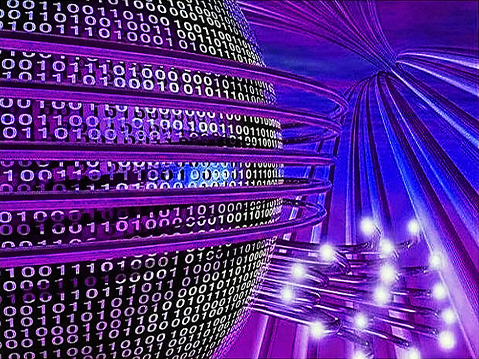
As I watched my one-month old baby sleeping, a thought ran through my mind. I wonder what technology would look like when she’s my age. There’s a lot of things going on simultaneously in technology today. I remember doing Artificial Intelligence/Machine Learning about 15 years ago. They used to be done in a university setting. They are now the new normal. Some technologies are quite recent like Big Data and Blockchain but they have become mainstream very quickly. I wonder what it will look like when my daughter grows up.

There is a technology I’m currently watching. It’s still in it’s infancy but this technology is really fascinating. It is a technology based on a remarkably counter-intuitive theory of the universe that governs the atoms and sub-atomic particles. It is called Quantum Computing. Given the high speed at which science fiction become realities, it’s possible that my baby girl will someday be programming on a quantum computer. But for now, we can only hope.

I have not seen a Quantum Computer and based on what I read so far, it’s still an engineering challenge. It might probably be a few more years before they are mass-produced but it is something to look forward to. But the good thing is, we can already talk about quantum algorithms! So let’s sharpen our pencils and get a few sheets of paper for we are going to talk about this new way of computing.

In classical computing, a bit has a value that is either one or zero. In quantum computing, a bit can now have a value that is a superposition of 1 and 0. We call this a QBit. The values 1 and 0 are now symbolized as $ \left\vert 1\right\rangle $ and $ \left\vert 0\right\rangle $ respectively. These are unit vectors in what is known as a Hilbert space. They are also known as kets, derived from the word bracket which we’ll talk more of later. An example of a vector space that you are familiar with is the color wheel. Each color is actually a combination of red, blue and green. For example, the color yellow is a combination of red and green. It’s also the same as with the qubit. A general QBit vector is of the form

\[\displaystyle \left| \Psi \right\rangle = a\left| 0\right\rangle + b\left| 1\right\rangle\]

such that $\mid a\mid^2 + \mid b\mid^2 = 1$. The numbers a and b are complex numbers and the symbol $\mid a\mid^2$ is defined as

\[\displaystyle \mid a\mid^2 = a^*a\]

where $a^*$ is the complex conjugate of a. A QBit vector represents the state of the QBit. We shall use the term vector and state interchangeably moving forward.

However, you won’t be able to see them in superposition state. If you want to know the state of a qubit, you will have to measure it. But when you measure it, it will collapse to one of either $\left\vert 0\right\rangle$ or $\left\vert 1\right\rangle$ but you will have a clue as to what that state will be. The coefficients a and b will give you the probability of the result of the measurement: it will be $\mid a\mid^2$ in state $\left\vert a\right\rangle$ and $\mid b\mid^2$ in state $\left\vert b\right\rangle$.

If the state of a QBit is a superposition of basis states $\left\vert 0\right\rangle$ and $\left\vert 1\right\rangle$, does this mean our computation is also random? Does it mean we get different answers every time ?

It turns out that we can get a definite answer! Let’s illustrate this by a simple quantum computation.

Suppose a I have a number between 0 and 1 million. What is my number? You can guess my number and I will only tell you if you got it correctly or not. I won’t tell you if my number is higher or lower than your guess. How many tries do you think you need in order to guess my number? I’m sure our tries will be many. In the worst case, you’ll need about 1 million tries.

For a quantum computer, you only need one try to guess it and that’s what we’re going to see. However, bear with me since we have to build up our arsenal of tools first before we can even talk about it. Let’s start with how a QBit looks like as a matrix.

The basis QBits $\left\vert 0\right\rangle$ and $\left\vert 1\right\rangle$ can be written as 1x2 matrices:

\[\displaystyle \left| 0 \right\rangle = \begin{bmatrix} 1\\ 0 \end{bmatrix}\] \[\displaystyle \left| 1 \right\rangle = \begin{bmatrix} 0\\ 1 \end{bmatrix}\]

Using this representation, we can write a general QBit as:

\[\displaystyle \mid\Psi\rangle = a\mid 0\rangle + b\mid 1\rangle = a \begin{bmatrix} 1\\ 0 \end{bmatrix} + b \begin{bmatrix} 0\\ 1 \end{bmatrix} = \begin{bmatrix} a\\ b \end{bmatrix}\]

So now we know that every QBit is a linear combination of ket vectors $\left\vert 0\right\rangle$ and $\left\vert 1\right\rangle$. These ket vectors have a corresponding “bra” vectors $\langle 0 \mid$ and $\langle 1\mid$. In matrix representation, the bra basis vectors are defined as:

\[\displaystyle \langle 0\mid = \begin{bmatrix} 1 & 0 \end{bmatrix}\]

and

\[\displaystyle \langle 1\mid = \begin{bmatrix} 0 & 1 \end{bmatrix}\]

For a general QBit $\mid\Psi\rangle = a\mid 0\rangle + b\mid 1\rangle$, the corresponding bra vector is

\[\displaystyle \langle \Psi \mid = a^*\langle 0\mid + b^*\langle 1\mid = \begin{bmatrix} a^* & b^* \end{bmatrix}\]

There is an operation between bra and ket vectors of the basis states called inner product which is defined as:

\[\begin{array}{rl} \displaystyle \langle 0\mid 0 \rangle &= 1\\ \displaystyle \langle 1\mid 1 \rangle &= 1\\ \displaystyle \langle 0\mid 1 \rangle &= \langle 1\mid 0\rangle = 0 \end{array}\]

Using the above rules, we can define the inner product of any two QBits $\mid \Psi\rangle = a\mid 0\rangle + b\mid 1\rangle$ and $\mid\Phi\rangle = c\mid 0\rangle + d\mid 1\rangle$ as

\[\begin{array}{rl} \displaystyle \langle \Psi\mid\Phi\rangle &= \big(a^*\langle 0\mid + b^*\langle 1\mid\big)\big(c\mid 0\rangle + d\mid 1\rangle\big)\\ &= \displaystyle a^*c \langle 0\mid 0\rangle + a^*\langle 0\mid 1\rangle + b^*c\langle 1\mid 0\rangle + b^*d\langle 1\mid 1\rangle\\ &= a^*c + b^*d \end{array}\]

Using the above definition of an inner product, the norm of a vector is defined as

\[\displaystyle \mid\left|\Psi\right\rangle\mid = \displaystyle \sqrt{\langle \Psi \mid \Psi \rangle} =\displaystyle \sqrt{a^*a + b^*b}\]

Geometrically, the norm is the length of the ket $\mid \Psi\rangle$.

Quantum computations are done using quantum operators. They are also called quantum gates. Operators are linear mappings that take a state to another state. That is, an operator $\mathbf{A}$ acts on $a\left\vert 0 \right\rangle + b\left\vert 1\right\rangle$ to give another vector $c\left\vert 0 \right\rangle + d\left\vert 1\right\rangle$. We write this as

\[\displaystyle \mathbf{A}(a\left\vert 0\right\rangle + b\left\vert 1\right\rangle) = c\left\vert 0\right\rangle + d\left\vert 1\right\rangle\]

Since the basis vectors $\left\vert 0\right\rangle$ and $\left\vert 1\right\rangle$ are also vectors, operators can also operate on them. An example of a very important operator and it’s action on the basis vectors is the Hadamard operator:

\[\begin{array}{rl} \displaystyle \mathbf{H} \left| 0 \right\rangle &= \displaystyle \frac{1}{\sqrt{2}}(\left| 0 \right\rangle + \left| 1\right\rangle)\\ \displaystyle \mathbf{H} \left| 1 \right\rangle &= \displaystyle \frac{1}{\sqrt{2}}(\left| 0 \right\rangle - \left| 1\right\rangle) \end{array}\]

By knowing the action of an operator on the basis vectors, we can determine the matrix representation of an operator. For the Hadamard operator, the matrix representations are:

\[\displaystyle \mathbf{H} \left| 0 \right\rangle = \displaystyle \frac{1}{\sqrt{2}}(\left| 0 \right\rangle + \left| 1\right\rangle) = \frac{1}{\sqrt{2}} \begin{bmatrix} 1\\ 1 \end{bmatrix}\]

and

\[\displaystyle \mathbf{H} \left| 1 \right\rangle = \displaystyle \frac{1}{\sqrt{2}}(\left| 0 \right\rangle - \left| 1\right\rangle) = \frac{1}{\sqrt{2}} \begin{bmatrix} 1\\ -1 \end{bmatrix}\]

Therefore the matrix representation of the Hadamard operator is

\[\displaystyle \mathbf{H}= \frac{1}{\sqrt{2}} \begin{bmatrix} 1 & 1 \\ 1 & -1 \end{bmatrix}\]

The identity operator is defined as the operator that maps a vector into itself and is symbolized as $\mathbf{I}$:

\[\displaystyle \mathbf{I}\left|\Psi\right\rangle = \left|\Psi\right\rangle\]

The NOT operator is defined as

\[\begin{array}{rl} \mathbf{X}\left|0\right\rangle &= \left|1\right\rangle\\ \mathbf{X}\left|1\right\rangle &= \left|0\right\rangle \end{array}\]

What it does is transform the $\left\vert 0\right\rangle$ to $\left\vert 1\right\rangle$ and vice versa, just like the classical bits.

Operators are linear. We can use linearity to derive the resulting vector when an operator acts on a general QBit:

\[\displaystyle \mathbf{A}(a\left| 0\right\rangle + b\left| 1\right\rangle) = a\mathbf{A} \left| 0\right\rangle + b\mathbf{A} \left| 1\right\rangle)\]

If $\mathbf{A}$ is the Hadamard operator, that is, $\mathbf{A} = \mathbf{H}$, then the above operation becomes:

\[\displaystyle \mathbf{H}(a\left| 0\right\rangle + b\left| 1\right\rangle) = a\mathbf{H} \left| 0\right\rangle + b\mathbf{H} \left| 1\right\rangle)\]

Since we know that:

\[\begin{array}{rl} \displaystyle \mathbf{H} \left| 0 \right\rangle &= \displaystyle \frac{1}{\sqrt{2}}(\left| 0 \right\rangle + \left| 1\right\rangle)\\ \displaystyle \mathbf{H} \left| 1 \right\rangle &= \displaystyle \frac{1}{\sqrt{2}}(\left| 0 \right\rangle - \left| 1\right\rangle) \end{array}\]

We can then write this as:

\[\begin{array}{rl} \displaystyle \mathbf{H}(a\left| 0\right\rangle + b\left| 1\right\rangle) &= \displaystyle a\mathbf{H} \left| 0\right\rangle + b\mathbf{H} \left| 1\right\rangle)\\ &= \displaystyle a\frac{1}{\sqrt{2}}\big(\left| 0\right\rangle + \left| 1\right\rangle\big) + b\frac{1}{\sqrt{2}}\big(\left| 0\right\rangle - \left| 1\right\rangle\big)\\ &= \displaystyle \frac{a+b}{\sqrt{2}} \left| 0\right\rangle + \frac{a-b}{\sqrt{2}} \left| 1\right\rangle \end{array}\]

Let see what the operators look like when they operate on bra vectors. Let’s start with the Hadamard operator acting on a general QBit above.

\[\begin{array}{rl} \displaystyle \mathbf{H} \mid 0 \rangle &= \displaystyle \frac{1}{\sqrt{2}}(\mid 0 \rangle + \mid 1\rangle) \rightarrow \langle 0\mid \mathbf{H^\dagger} = \displaystyle \frac{1}{\sqrt{2}}(\langle 0 \mid + \langle 1\mid)\\ \displaystyle \mathbf{H} \mid 1 \rangle &= \displaystyle \frac{1}{\sqrt{2}}(\mid 0 \rangle - \mid 1\rangle) \rightarrow \langle 1\mid \mathbf{H^\dagger} = \displaystyle \frac{1}{\sqrt{2}}(\langle 0 \mid - \langle 1\mid) \end{array}\]

where we symbolize $\mathbf{H^\dagger}$ as the operator corresponding to the Hadamard operator acting on bras.

The matrix representation of the Hadamard operator acting on bras is therefore:

\[\mathbf{H^\dagger} = \frac{1}{\sqrt{2}} \begin{bmatrix} 1 & 1\\ 1 & -1 \end{bmatrix} = \mathbf{H}\]

In general, the matrix representation of $\mathbf{H^\dagger}$ is the conjugate transpose of the matrix of $\mathbf{H}$. In simple terms, this means take the transpose of $\mathbf{H}$ and apply the complex conjugates to each element. It’s amazing that the Hadamard operator is equal to its conjugate transpose. The types of operators that behave that way are called Hermitian operators.

Let $\mathbf{A}$ be an operator and $\left\vert \Psi\right\rangle$ a vector and let $\Phi = \mathbf{A}\left\vert\Psi\right\rangle$, then the norm of $\Phi$ is

\[\displaystyle \langle\Phi\mid\Phi\rangle = \langle \Psi\mid \mathbf{A^\dagger}\mathbf{A}\mid \Psi\rangle = \langle\Psi\mid\Psi\rangle\]

This means that

\[\displaystyle \mathbf{A^\dagger}\mathbf{A} = \mathbf{I}\]

The kind of operator that satisfies the above relationship is called Unitary.

Now that we have gained knowledge of some of the tools, we can now describe how a quantum computation is set up. We need QBits for the input and QBits for the output. The simplest setup is a one QBit input and one QBit output. Let $\left\vert x\right\rangle$ and $\left\vert y\right\rangle$ be the input and output QBits,respectively. The general state of this quantum system is a superposition of the following states:

\[\left| 0 \right\rangle \otimes \left| 0 \right\rangle, \left| 0 \right\rangle \otimes \left| 1 \right\rangle, \left| 1 \right\rangle \otimes \left| 0 \right\rangle, \left| 1 \right\rangle \otimes \left| 1 \right\rangle\]

which could also be written as

\[\left|00\right\rangle, \left|01\right\rangle, \left|10\right\rangle, \left|11\right\rangle,\]

or, if we take them as binary representation of numbers, we can write them concisely as

\[\left|0\right\rangle, \left|1\right\rangle,\left|2\right\rangle,\left|3\right\rangle,\]

Using the above basis vectors, we can write a general 2-QBit system as:

\[\displaystyle \left|\Psi\right\rangle = c_1\left|0\right\rangle + c_1\left|1\right\rangle + c_1\left|2\right\rangle + c_1\left|3\right\rangle = \sum_{i=0}^{2^n-1} c_i\left|i\right\rangle\]

where the numbers $c_i$ are complex and n=2. The summation is up to $2^n-1$ since the maximum number n QBits can represent is $2^n-1$. The summation on the right also gives us the general form of a QBit for an n-QBit system.

As we saw earlier, the quantum operators (or gates) are the ones used to compute from a given QBit inputs. Let $\mathbf{U}_f$ represent a unitary operator implementing the function f. The function f is a function that takes the numbers from the domain ${0,1}$ to ${0,1}$, that is,

\[\displaystyle f: \{0,1\}\rightarrow \{0,1\}\]

For a two-QBit system, the form of quantum computation is

\[\displaystyle \mathbf{U}_f\left|x\right\rangle \left|y\right\rangle = \left|x\right\rangle \left|x\oplus f(x)\right\rangle\]

where the symbol $\oplus$ represent bitwise OR operation. The table below will give you the results of the bitwise OR operation for every combination of values in ${0,1}$:

\[\begin{array}{cc} 0 \oplus 0 &= 0\\ 0 \oplus 1 &= 1\\ 1 \oplus 0 &= 1\\ 1 \oplus 1 &= 0 \end{array}\]

A simple but important example of a unitary operator acting on two QBits is the $\mathbf{C_{\text{NOT}}}$ gate, defined as:

\[\displaystyle \mathbf{C_{\text{NOT}}}\left|x\right\rangle\left|y\right\rangle = \left|x\right\rangle\left|y \oplus x\right\rangle\]

Here is the complete action of the $\mathbf{C_{\text{NOT}}}$:

\[\begin{array}{c|c|c} \text{Input} & \text{Output} & \text{Result}\\ 0 & 0 & 0\\ 0 & 1 & 1\\ 1 & 0 & 1\\ 1 & 1 & 0 \end{array}\]

If you study the table above, you’ll notice that if the input QBit is in the state $\left\vert 0\right\rangle$, the output QBit stays the same. However, if the input QBit is in $\left\vert 1\right\rangle$, the output QBit is flipped. The input QBit in this case controls the flipping of the second QBit. The input QBit is said to be the control bit. That’s why it’s called a $\mathbf{C_{\text{NOT}}}$ which stands for Controlled-NOT gate.

Let’s now go back to our original problem. There is a positive number $a$ that is less than $2^n$ . We want to find this number using quantum computation. We are given a black box operator $\mathbf{U}_f$ whose action on a bra is

\[\displaystyle \mathbf{U}_f \left|x\right\rangle\left|y\right\rangle = \left|x\right\rangle\left| y \oplus f(x)\right\rangle\]

where

\[\displaystyle f(x) = x_0 a_0 \oplus x_1 a_1 \oplus \cdots x_{n-1}a_{n-1} = x \cdot a\]

where $a$ is the unknown number we are going to guess and $x_ia_i$ are the i-th bits of x and a.

So how many times do we have to apply $\mathbf{U}_f$ in order to guess the number $a$?

To solve this, we need $n$ input QBits and 1 output QBit. We will initialize our QBits to $\left\vert 0\right\rangle$. So the initial configuration is

\[\displaystyle \underbrace{\left|000...0\right\rangle}_{\text{n number of zeroes}}\otimes\left|1\right\rangle\]

Notice how we separate the input and output qubits.

Next we apply the Hadamard operator to each QBit:

\[\displaystyle \mathbf{H}^{\otimes n}\otimes \mathbf{H} \left|000...0\right\rangle\left|1\right\rangle = \mathbf{H}^{\otimes n} \left|000...0\right\rangle\otimes \mathbf{H}\left|1\right\rangle\]

We have seen the Hadamard operator earlier. For the sake of convenience we’ll repeat it here:

\[\begin{array}{rl} \displaystyle \mathbf{H} \left| 0 \right\rangle &= \displaystyle \frac{1}{\sqrt{2}}(\left| 0 \right\rangle + \left| 1 \right\rangle)\\ \displaystyle \mathbf{H} \left| 1 \right\rangle &= \displaystyle \frac{1}{\sqrt{2}}(\left| 0 \right\rangle - \left| 1\right\rangle) \end{array}\]

We can generalize this by letting x be either 0 or 1:

\[\begin{array}{rl} \displaystyle \mathbf{H}\left| x\right\rangle &= \frac{1}{\sqrt{2}}\big(\left|0\right\rangle + (-1)^x \left|1\right\rangle \end{array}\]

We can use this to compute the action on two QBits and generalize:

\[\begin{array}{rl} \displaystyle \mathbf{H}^{\otimes 2}\left| x\right\rangle &= \mathbf{H}^{\otimes 2}\left| x_0x_1\right\rangle = \mathbf{H}\left| x_0\right\rangle \otimes \mathbf{H}\left| x_1\right\rangle\\ &= \displaystyle \frac{1}{\sqrt{2}}\big(\left|0\right\rangle + (-1)^{x_0} \left|1\right\rangle \otimes \frac{1}{\sqrt{2}}\big(\left|0\right\rangle + (-1)^{x_1} \left|1\right\rangle\\ &= \displaystyle \big(\frac{1}{\sqrt{2}}\big)^2 \big( \left|00\right\rangle + (-1)^{x_0} \left|01\right\rangle + (-1)^{x_1}\left|10\right\rangle + (-1)^{x_1 + x_0}\left|11\right\rangle\\ &= \displaystyle \big(\frac{1}{\sqrt{2}}\big)^2 \big( (-1)^{0\cdot x_1 + 0\cdot x_0} \left|00\right\rangle + (-1)^{0\cdot x_1 + 1\cdot x_0} \left|01\right\rangle + (-1)^{1\cdot x_1 + 0\cdot x_0}\left|10\right\rangle + (-1)^{1\cdot x_1 + 1\cdot x_0}\left|11\right\rangle\\ &= \displaystyle \big(\frac{1}{\sqrt{2}}\big)^2 \big( (-1)^{0\cdot x_1 + 0\cdot x_0} \left|0\right\rangle + (-1)^{0\cdot x_1 + 1\cdot x_0} \left|1\right\rangle + (-1)^{1\cdot x_1 + 0\cdot x_0}\left|2\right\rangle + (-1)^{1\cdot x_1 + 1\cdot x_0}\left|3\right\rangle\\ &= \displaystyle \big(\frac{1}{\sqrt{2}}\big)^2 \sum_{y=0}^{2^2-1} (-1)^{x\cdot y}\left|y\right\rangle \end{array}\]

In general,

\[\displaystyle \mathbf{H}^{\otimes n}\left| x\right\rangle = \frac{1}{2^{n/2}}\sum_{y=0}^{2^n-1} (-1)^{x\cdot y}\left|y\right\rangle\]

Using the above formula, the action of $\mathbf{H}^{\otimes n}$ on $\left\vert 0\right\rangle$ is

\[\displaystyle \mathbf{H}^{\otimes n} \left|0\right\rangle = \frac{1}{2^{n/2}}\sum_{y=0}^{2^n-1} \left|y\right\rangle\]

The next step is to apply our operator $\mathbf{U}_{f}$ which was defined above:

\[\begin{array}{rl} \displaystyle \mathbf{U}_f\mathbf{H}^{\otimes n}\left| 0\right\rangle \otimes \frac{1}{\sqrt{2}} \big( \left|0\right\rangle - \left|1\right\rangle\big) &= \displaystyle \frac{1}{2^{n/2}}\sum_{y=0}^{2^n-1} \mathbf{U}_f\left|y\right\rangle \otimes \frac{1}{\sqrt{2}} \big( \left|0\right\rangle - \left|1\right\rangle\big)\\ &= \displaystyle \frac{1}{2^{n/2}}\sum_{y=0}^{2^n-1} \frac{1}{\sqrt{2}} \big( \mathbf{U}_f\left|y\right\rangle \otimes \left|0\right\rangle - \mathbf{U}_f\left|y\right\rangle \otimes \left|1\right\rangle\big)\\ &= \displaystyle \frac{1}{2^{n/2}}\sum_{y=0}^{2^n-1} \frac{1}{\sqrt{2}} \big( \left|y\right\rangle \otimes \left|0\oplus f(y)\right\rangle - \left|y\right\rangle \otimes \left|1\oplus f(y)\right\rangle\big)\\ \end{array}\]

Let’s break this down a bit. Since the value of $f(y)$ is either 0 or 1, we have 2 cases:

When $f(y) = 0$,

\[\displaystyle \left|y\right\rangle \otimes \left|0\oplus f(y)\right\rangle = \left|y\right\rangle \otimes \left|0\right\rangle\] \[\displaystyle \left|y\right\rangle \otimes \left|1\oplus f(y)\right\rangle = \left|y\right\rangle \otimes \left|1\right\rangle\]

which means

\[\displaystyle \frac{1}{2^{n/2}}\sum_{y=0}^{2^n-1} \frac{1}{\sqrt{2}} \big( \left|y\right\rangle \otimes \left|0\oplus f(y)\right\rangle - \left|y\right\rangle \otimes \left|1\oplus f(y)\right\rangle\big) = \frac{1}{2^{n/2}}\sum_{y=0}^{2^n-1} \left|y\right\rangle \otimes \frac{1}{\sqrt{2}} \big( \left|0\right\rangle - \left|1\right\rangle\big)\]

When $f(y) = 1$,

\[\displaystyle \left|y\right\rangle \otimes \left|0\oplus f(y)\right\rangle = \left|y\right\rangle \otimes \left|1\right\rangle\] \[\displaystyle \left|y\right\rangle \otimes \left|1\oplus f(y)\right\rangle = \left|y\right\rangle \otimes \left|0\right\rangle\]

which means

\[\displaystyle \frac{1}{2^{n/2}}\sum_{y=0}^{2^n-1} \frac{1}{\sqrt{2}} \big( \left|y\right\rangle \otimes \left|0\oplus f(y)\right\rangle - \left|y\right\rangle \otimes \left|1\oplus f(y)\right\rangle\big) = \frac{1}{2^{n/2}}\sum_{y=0}^{2^n-1} (-1) \left|y\right\rangle \otimes \frac{1}{\sqrt{2}} \big( \left|0\right\rangle - \left|1\right\rangle\big)\]

Combining these 2 we have

\[\begin{array}{rl} \displaystyle \mathbf{U}_f\mathbf{H}^{\otimes n}\left| 0\right\rangle \otimes \frac{1}{\sqrt{2}} \big( \left|0\right\rangle - \left|1\right\rangle\big) &= \displaystyle \frac{1}{2^{n/2}}\sum_{y=0}^{2^n-1} \frac{1}{\sqrt{2}} \big( \left|y\right\rangle \otimes \left|0\oplus f(y)\right\rangle - \left|y\right\rangle \otimes \left|1\oplus f(y)\right\rangle\big)\\ &= \displaystyle \frac{1}{2^{n/2}}\sum_{y=0}^{2^n-1} (-1)^{f(y)} \left|y\right\rangle \otimes \frac{1}{\sqrt{2}} \big( \left|0\right\rangle - \left|1\right\rangle\big) \end{array}\]

Finally, getting the Hadamard action on this gives:

\[\begin{array}{rl} \displaystyle \mathbf{H}^{\otimes n}\otimes\mathbf{H}\Big[\mathbf{U}_f\mathbf{H}^{\otimes n}\left| 0\right\rangle \otimes \frac{1}{\sqrt{2}} \big( \left|0\right\rangle - \left|1\right\rangle\big)\Big] &=\mathbf{H}^{\otimes n} \mathbf{U}_f\mathbf{H}^{\otimes n}\left| 0\right\rangle \otimes \mathbf{H}\Big[\frac{1}{\sqrt{2}} \big( \left|0\right\rangle - \left|1\right\rangle\big)\Big]\\ &= \underbrace{\mathbf{H}^{\otimes n} \Big[\displaystyle \frac{1}{2^{n/2}}\sum_{y=0}^{2^n-1} (-1)^{f(y)} \left|y\right\rangle \Big]}_{A} \otimes \underbrace{\mathbf{H}\Big[\frac{1}{\sqrt{2}} \big( \left|0\right\rangle - \left|1\right\rangle\big)\Big]}_{B} \end{array}\]

Expanding underbrace B gives us:

\[\begin{array}{rl} \displaystyle \mathbf{H}\Big[\frac{1}{\sqrt{2}} \big( \left|0\right\rangle - \left|1\right\rangle\big)\Big] &= \displaystyle \frac{1}{\sqrt{2}}\big(\mathbf{H}\left|0\right\rangle - \mathbf{H}\left|1\right\rangle\big)\\ &= \displaystyle \frac{1}{\sqrt{2}}\Big[\frac{1}{\sqrt{2}} \big( \left|0\right\rangle + \left|1\right\rangle \big) - \frac{1}{\sqrt{2}}\big( \left|0\right\rangle - \left|1\right\rangle\big) \Big]\\ &= \displaystyle \frac{1}{2}\Big[ 2\left|1\right\rangle \Big]\\ &= \left|1\right\rangle \end{array}\]

Expanding underbrace A above:

\[\begin{array}{rl} \mathbf{H}^{\otimes n} \Big[\displaystyle \frac{1}{2^{n/2}}\sum_{y=0}^{2^n-1} (-1)^{f(y)} \left|y\right\rangle \Big] &= \displaystyle \frac{1}{2^{n/2}}\sum_{y=0}^{2^n-1} (-1)^{f(y)}\mathbf{H}^{\otimes n} \left|y\right\rangle \end{array}\]

We have found earlier that

\[\displaystyle \mathbf{H}^{\otimes n}\left| y\right\rangle = \frac{1}{2^{n/2}}\sum_{x=0}^{2^n-1} (-1)^{x\cdot y}\left|x\right\rangle\]

Substituting this to the above and noting that

\[\displaystyle f(y) = y\cdot a = \sum_{i=0}^{n-1} y_ia_i \mod 2\]

we get:

\[\begin{array}{rl} \mathbf{H}^{\otimes n} \Big[\displaystyle \frac{1}{2^{n/2}}\sum_{y=0}^{2^n-1} (-1)^{f(y)} \left|y\right\rangle \Big] &= \displaystyle \frac{1}{2^{n/2}}\sum_{y=0}^{2^n-1} (-1)^{f(y)}\mathbf{H}^{\otimes n} \left|y\right\rangle \\ &= \displaystyle \frac{1}{2^{n}}\sum_{y=0}^{2^n-1} \sum_{x=0}^{2^n-1} (-1)^{f(y)}(-1)^{y\cdot x}\left|x\right\rangle\\ &= \displaystyle \frac{1}{2^{n}}\sum_{y=0}^{2^n-1} \sum_{x=0}^{2^n-1} (-1)^{y\cdot a}(-1)^{y\cdot x}\left|x\right\rangle\\ &= \displaystyle \frac{1}{2^{n}}\sum_{x=0}^{2^n-1} \underbrace{\sum_{y=0}^{2^n-1} (-1)^{(a+x)\cdot y}}\left|x\right\rangle\\ \end{array}\]

where we have interchanged the order of the summation. To simplify the term with the underbrace, notice that

\[\begin{array}{rl} \displaystyle \Big[1+ (-1)^{z_0}\Big]\Big[1+(-1)^{z_1}\Big] &= 1 + (-1)^{z_0} + (-1)^{z_1} + (-1)^{z_0+z_1}\\ &= \displaystyle (-1)^{0\cdot z_0 + 0\cdot z_1} + (-1)^{1\cdot z_0 + 0\cdot z_1} + (-1)^{0\cdot z_0 + 1\cdot z_1} + (-1)^{1\cdot z_0+ 1\cdot z_1}\\ &= \displaystyle(-1)^{0\cdot z} + (-1)^{1\cdot z} + (-1)^{2\cdot z} + (-1)^{3\cdot z}\\ &= \displaystyle \sum_{y=0}^{2^2-1} (-1)^{y\cdot z} \end{array}\]

We can therefore write the factor in underbrace as

\[\begin{array}{rl} \mathbf{H}^{\otimes n} \Big[\displaystyle \frac{1}{2^{n/2}}\sum_{y=0}^{2^n-1} (-1)^{f(y)} \left|y\right\rangle \Big] &= \displaystyle \frac{1}{2^{n}}\sum_{x=0}^{2^n-1} \underbrace{\sum_{y=0}^{2^n-1} (-1)^{(a+x)\cdot y}}\left|x\right\rangle\\ &= \displaystyle \frac{1}{2^{n}}\sum_{x=0}^{2^n-1} \prod_{i=0}^{n-1} \Big[ \underbrace{1 +(-1)^{(a_i+x_i)}}\Big] \left|x\right\rangle\\ \end{array}\]

Notice that

\[\displaystyle 1 +(-1)^{(a_i+x_i)} = \begin{cases} 0 & x\ne a\\ 2 & x=a \end{cases}\]

that is, the product $\prod_{i=0}^{n-1} \Big[1 + (-1)^{(a_i+x_i)}\Big] = 0$ unless $x=a$. Therefore

\[\begin{array}{rl} \mathbf{H}^{\otimes n} \Big[\displaystyle \frac{1}{2^{n/2}}\sum_{y=0}^{2^n-1} (-1)^{f(y)} \left|y\right\rangle \Big] &= \displaystyle \frac{1}{2^{n}}\sum_{x=0}^{2^n-1} \prod_{i=0}^{n-1} \Big[ \underbrace{1 +(-1)^{(a_i+x_i)}}\Big] \left|x\right\rangle\\ &= \displaystyle \frac{1}{2^{n}} 2^n \left|a\right\rangle\\ &= \left|a\right\rangle \end{array}\]

Therefore, the quantum computation gives the answer in one application of $\mathbf{U}_f$:

\[\displaystyle \mathbf{H}^{\otimes n+1}\mathbf{U}_f \mathbf{H}^{\otimes n+1} \left|0\right\rangle = \left| a\right\rangle \left| 1\right\rangle\]

So what just happened? We began with a superposition of states and finished with the correct answer in one application of the black box operator $\mathbf{U}_f$. That’s the power of Quantum Computing!

Image Credit: “Quantum Computing” by arkhangellohim is marked with CC BY-NC-SA 2.0. To view the terms, visit https://creativecommons.org/licenses/by-nc-sa/2.0/?ref=openverse